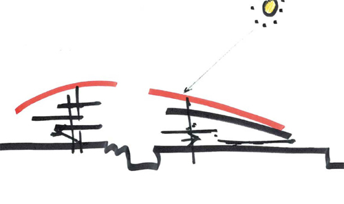
To simulate an incompressible, steady-state, turbulent flow over a double-sided membrane. View velocity vectors, velocity magnitude color maps, monitor lift and drag forces, and export results for ixForten 4000.
Caedium Membrane CFD Simulation
Goals
In this tutorial, you will learn how to:
- Specify fluid conditions on a single volume for an incompressible, steady-state, turbulent flow simulation
- Specify boundary conditions on faces
- Specify meshing parameters
- Generate a velocity magnitude color map
- Generate velocity vectors
- Create lift and drag force monitors
- Monitor residuals to determine flow simulation convergence
- Export results for ixForten 4000
Assumptions
- You have activated the Caedium RANS Flow and Viz Export add-ons, or Caedium Professional.
- You are familiar with Caedium essentials.
-
You have either:
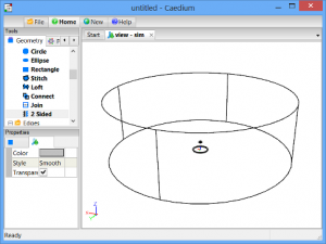
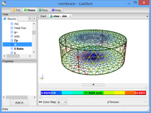
The geometry within Caedium should appear as shown below.
Prepare the Volume
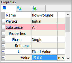
Right-click an edge of the volume, double-click the first volume (volume_2) in the Select dialog and then select Properties from the menu. In the Properties Panel, select the Volume tab  and set theName to flow-volume.
Create Membrane Group
Create a group for the membrane and its shadow so that later on in this tutorial you can monitor the integrated drag and lift forces.
Right click on the membrane base edge. In the Select dialog selectface_6-shadow, press the Ctrl key and select face_6 in the Selectdialog, click OK, select Group, and then select Properties.
In the Properties Panel, select the Group tab and set Name tomembrane.
Specify the Substance Settings
Specify the Fluid Conditions
Select the Physics Tool Palette. Select Substances->Air. The Properties Panel will show the default properties for air. To enable incompressible turbulent (viscous) flow the State->Rotational and State->Viscousproperties should be set to Yes (their default values), and the State->Compressible, State->Heat Transfer and State->Transient properties should to be set to No (their default values).
Drag and drop the Substances->Air tool onto an edge of the volume. Select Done to set air as the fluid inside the volume.
Set the Reference Velocity for the Simulation
The reference velocity will be used to initialize the simulation and to specify the free stream velocity boundary condition. In this tutorial you will set a reference velocity of [8.66 5 0] m.s-1, from 10 m.s-1 @ theta = 30 degrees to give [10 * cos(30), 10 * sin(30), 0].
In the Properties Panel set Substance: Air->Properties->Phase: Single->Reference->U: Fixed Value->Value to be [8.66 5 0] and press Enter on the keyboard.
Set the Non-Orthogonal Corrections for the Simulation
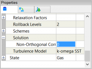
In the Properties Panel, expand the Substance: Air->Solver: RANS Flow->Solution property, and then set Non-Orthogonal Corrections to be 0.
Specify the Boundary Conditions
Wall Conditions
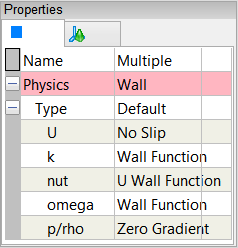
Drag and drop the Conditions->Wall tool onto an edge of the volume. Double-click flow-volume->Faces in the Select dialog and select Doneto create walls on the outer surfaces of the volume.
A Wall condition is a solid surface through which fluid cannot flow.
Inlet-Outlet Conditions
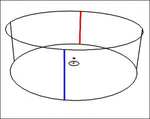
Drag and drop the Conditions->Inlet-Outlet tool onto edge_8 (blue). In the Select dialog select face_1, press Ctrl and select face_5 in theSelect dialog, click OK, and select Select/Deselect. Select edge_7 (red) in the View Window, in the Select Dialog select face, press Ctrl and select face_4, click OK, select Group, and select Done.
In the Properties Panel, set Name to be circumference, and set Physics: Inlet-Outlet->Type to be Free Stream.
An Inlet-Outlet condition of type Free Stream allows the fluid to enter or leave the flow domain.
Slip Condition
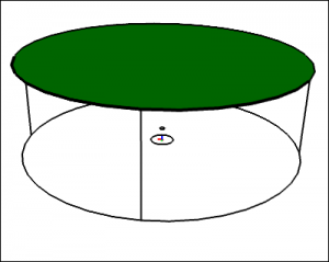
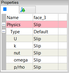
Drag and drop the Conditions->Slip tool onto an edge of the face shown in green below, double-click face_3 in the Select dialog and select Done.
A Slip condition ensures the flow velocity remains tangential to a face.
Specify Meshing Parameters
You do not need to apply any volume or boundary condition prior to focusing on the meshing process – all that is required is an active Substance on your flow domain.
Face Mesh
First you will focus on the surface mesh to avoid the extra time required to create the volume mesh.
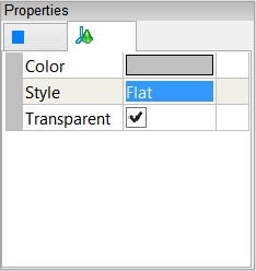
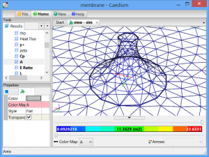
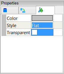
To see individual surface mesh elements during the meshing process, right-click on the View Window background, double-click sim->Faces, and select Properties from the menu. In the Properties Panel, set Style toFlat.
Select the Results Tool Palette. With all faces still selected from the previous operation select the Scalar Fields->A (area) tool, click Add A at the bottom of the Properties Panel and select Color Map.
The request for the A color map will cause all the faces to be meshed.
Zoom the view using the mouse wheel to focus on the membrane mesh.
Select the Physics Tool Palette and select the Conditions->Accuracytool. In the Properties Panel set Accuracy to Custom and set Resolutionto 100. Drag and drop the Conditions->Accuracy tool onto a membrane edge, double-click face_6 in the Select dialog, and select Done.
Applying the Accuracy tool will cause all the faces to be remeshed which will take a few seconds.
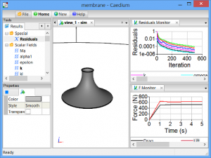
Volume Mesh
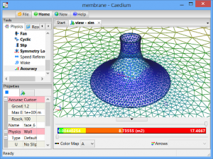
To see individual volume mesh elements during the meshing process, right-click on any edge in the View Window, double-click flow-volume, and select Properties from the menu. In the Properties Panel, turn off theTransparent property and set Style to Flat.
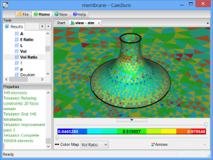
Select the Results Tool Palette. With the volume still selected from the previous operation double-click the Scalar Fields->Vol Ratio (volume ratio = actual volume/ideal volume) and select Color Map.
The request for the Vol Ratio color map will cause the entire volume to be meshed which will take a few seconds.
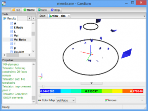
Drag the upper threshold slider to the left in the View Legend to examine the cells with the lowest quality (lowest value in the blue range).
If you were to see clusters of low quality cells attached to the geometry then that is a sign that you need to improve the mesh in that region using the Accuracy tool. Fortunately this mesh does not suffer from low quality element clusters and you can proceed on with the simulation.
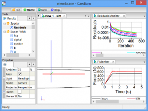
Display Initial Velocity Color Map
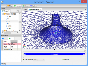
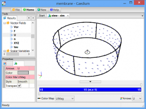
Drag and drop the Vector Fields->U (velocity) tool onto the View Window (view) background, double-click sim->Faces, select Color Map to create contours of velocity magnitude on all faces.
In the Properties Panel, set Style to Smooth.
Check that the velocity magnitude value (shown in the View Legend color bar) matches the value you expect as confirmation that your reference velocity is correct.
Display Initial Velocity Vectors
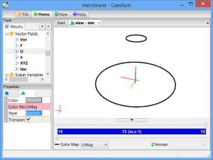
Drag and drop the Vector Fields->U (velocity) tool onto an edge of the circumference faces, double-click the circumference group in the Selectdialog, and select Arrows to create arrows colored by velocity magnitude.
Check that the arrows are oriented in the direction you expect as confirmation that your reference velocity is correct.
Create New Drag Result
Given that the air direction for this simulation can vary, i.e., it is not aligned with the X-axis, you need to create a new result for the drag force = Sum(F:X.Cos(theta) + F:Y.Sin(theta)), where F is force per element and theta is the angle between the air direction and the X-axis in the XY-plane.
The steps to calculate the new drag result are:
- Create a scalar constant theta
- Create Cos(theta) and Sin(theta)
- Create F:X.Cos(theta) and F:Y.Sin(theta)
- Create F:X.Cos(theta) + F:Y.Sin(theta)
- Create Sum(F:X.Cos(theta) + F:Y.Sin(theta))
Create Scalar Constant theta
In the Toolbar, click the New button and select Result.
In the Create Result dialog, select the Constant tab. For Units, selectAngle.
Click Create to create a scalar.
In the Results Tool Palette, select Scalar Variables->Scalar (the scalar variable you just created), click on it again to make its name editable, and change Scalar to theta.
In the Properties Panel, set the Value of theta to 30. Press Enter on the keyboard to apply the changes to the Properties Panel.
Create Sin(theta) and Cos(theta)
In the Create Result dialog, select the Unary tab. Select Sin from the list. Drag Scalar Variables->theta from the Results Tool Palette and drop it onto the target in the Create Result dialog and click Create to createSin(theta).
Perform the same procedure again but select Cos from the Unary operators list to create Cos(theta).
Create F:X.Cos(theta) and F:Y.Sin(theta)
In the Create Result dialog, select the Binary tab. Select Multiply from the list.
In the Results Tool Palette, select Vector Fields->F (force). In the Properties Panel set Scalar to X.
Drag and drop Vector Fields->F onto the left-hand target in the Create Result dialog. Select Scalar to specify the X-force-component as the left-hand variable for the equation.
Drag Scalar Variables->Cos(theta) from the Results Tool Palette and drop it onto the right-hand target in the Create Result dialog and clickCreate to create (F:X x Cos(theta)).
In the Results Tool Palette, select Vector Fields->F (force). In the Properties Panel set Scalar to Y.
Drag and drop Vector Fields->F onto the left-hand target in the Create Result dialog. Select Scalar to specify the Y-force-component as the left-hand variable for the equation.
Drag Scalar Variables->Sin(theta) from the Results Tool Palette and drop it onto the right-hand target in the Create Result dialog and clickCreate to create (F:Y x Sin(theta)).
Create F:X.Cos(theta) + F:Y.Sin(theta)
In the Create Result dialog, select the Binary tab. Select Add from the list.
Drag and drop Scalar Fields->(F:X x Cos(theta)) onto the left-hand target in the Create Result dialog. Drag and drop Scalar Fields->(F:Y x Sin(theta)) onto the right-hand target in the Create Result dialog and clickCreate to create ((F:X x Cos(theta)) + (F:Y x Sin(theta))).
Create Sum(F:X.Cos(theta) + F:Y.Sin(theta))
In the Create Result dialog, select the Unary tab. Select Sum from the list. Drag Scalar Fields->((F:X x Cos(theta)) + (F:Y x Sin(theta))) from the Results Tool Palette and drop it onto the target in the Create Resultdialog and click Create to create Sum(((F:X x Cos(theta)) + (F:Y x Sin(theta)))).
Close the Create Result dialog. In the Results Tool Palette, select Scalar Variables->Sum(((F:X x Cos(theta)) + (F:Y x Sin(theta)))) and rename itDrag.
Create Force Monitors
Drag Monitor
Drag and drop the Scalar Variables->Drag tool onto a membrane edge. Double-click the membrane group in the Select dialog and selectMonitor.
Drag and drop the Drag Monitor tab over to the right-hand edge of the Caedium application window to split the window into two parts as shown below.
Lift Monitor
In the Results Tool Palette, select Vector Variables->F (force). In the Properties Panel set Scalar to Z.
With the membrane group still selected from the previous Drag monitor creation, double-click the Vector Variables->F tool and select Monitor.
Drag and drop the F Monitor tab over to the right-hand edge of the Caedium application window to split the window into three parts as shown below.
Create Residuals Monitor
Left-click in the View Window to give it focus. Drag and drop the Special->Residuals tool onto a membrane edge. Double-click flow-volume in theSelect dialog and select Monitor to create the residuals monitor.
Drag and drop the Residuals Monitor tab over to the top-right-hand edge of the Caedium application window to add the monitor to the drag monitor tab row as shown below.
Run the Flow Solver
The number of flow (simulation) solver iterations is determined by multiplying the number of simulation time-steps (default = 5) by the number of iterations per simulation time-step (default = 100). The number of simulation time-steps is determined by dividing the simulation duration (default = 5 s) by the simulation time-step (default = 1 s). After each simulation time-step (equivalent to 100 iterations by default) the results will be refreshed. For this simulation the defaults are fine and will result in a total of 500 iterations.
To run the flow solver, click Play on the Toolbar.
If you wanted to interrupt the flow solver, you would re-click the Play button; the solver would then stop at the end of the current simulation time-step.
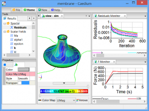
Let the solver complete its run. Note the updates of the velocity vectors, velocity color map, the forces monitors, and the residuals monitor as the simulation progresses.
Solver convergence is indicated by:
- The Residuals Monitor shows the solver residuals decreased with increasing iterations smoothly and progressed below 0.001, i.e., over 3 orders of magnitude reduction
- The Drag and F monitors both show convergence close to single values with increasing iterations
To make it easier to differentiate between the inner and outer membrane results, select the membrane base edge, in the Select dialog double-clickface_6 (inner results), and select Properties. In the Properties Panel, turn off the Transparent property.
If you change the reference velocity flow direction then you will also need to change theta used by the drag monitor. Select the View Window background, in the Select dialog double-click sim. In the Properties Panel select the Simulation tab and set Constants->theta accordingly.
Export Results to ixForten 4000
ixForten 4000 can import CFD results from Caedium as Alias/Wavefront (.obj) for the geometry and as Comma Separated Values (CSV) for the Pressure Coefficient (Cp) data.
Create New View
Click the New button on the toolbar and select View to create view_1.
Export the Membrane as .obj
Select the membrane base edge, in the Select dialog double-click face_6, and select Properties. In the Properties Panel turn off the Transparentproperty.
Right click on the View Window (view_1) background, in the Select dialog select sim->Edges, press the Ctrl key and select sim->Axes in theSelect dialog, and click OK. In the Properties Panel turn on theTransparent property.
This should leave only the membrane face visible ready for export.
In the Menu Bar, select File->Export…. In the Export dialog set Save as type to Alias/Wavefront (*.obj), set the File name to membrane-cp.obj, and click Save.
In addition to the membrane-cp.obj file the export operation will also save a membrane-cp.mtl file.
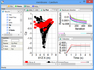
Export Cp Data as .csv
Drag and drop the Scalar Fields->Cp (pressure coefficient) tool onto the shaded membrane face in view_1. In the Select dialog double-click themembrane group, and select XY Plot to create a plot of the Cp values on the membrane faces.
Select File->Export…. In the Export dialog set Save as type to Plot Series (*.csv), set the File name to membrane-cp.csv, and click Save.


 and set theName to flow-volume.
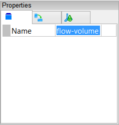
 and set Name tomembrane.
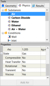

 and select Result.
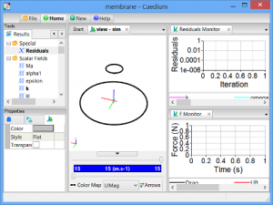
 on the Toolbar.
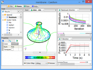
 and set Constants->theta accordingly.